In this project, I am going to perform the development of a linear regression model for salary prediction. It is pretty simple. It is meant as a revisal of the topic or simply a tutorial.
Data Set and the code: github.com/ilkecandan/Linear-Regression---S..
First of all; what is regression? And, how it is different from classification. Classification is done on discrete data, whereas regression is done on continuous data. Regression can be used to predict anything, including a person's age, a price, or the value of any variable. Predicting what class something belongs to is part of classification (such as whether a tumor is benign or malignant).
As usual, we will start with exploratory data analysis. We want to understand our data. In our data set, we have two values for years of experience and salary. So, we want to get to know them a little more. Let's import necessary libraries.
import pandas as pd
import numpy as np
import matplotlib.pyplot as plt
import seaborn as sns
import statsmodels.api as sm
from sklearn.model_selection import train_test_split
from sklearn.linear_model import LinearRegression
from sklearn.metrics import r2_score

sns.set()
%matplotlib inline

df = pd.read_csv("salar.csv")
Then, one by one, we should execute other commands.
df.head()
df.shape
df.isnull().values.any()
In general, understanding the shape of your data is essential to being able to analyze it and create models using it. Also, we don't have any empty values. It's great.
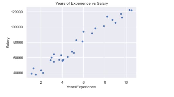
df.plot.scatter(x='YearsExperience', y='Salary', title=' Years of Experience vs Salary');

The salary rise as the number of years of experience does. There is a large positive link between these two! We claim that there is a positive linear correlation between the salary and years of experience variables because it looks that the form of the line the points are creating is straight. How closely are they related? In a DataFrame, the corr() function computes and shows the correlations between numerical variables:
print(df.corr())
print(df.describe())
From this function we can see avarage salary is 76003.000000.
Linear Regression
Preprocessing of Data
We previously imported Pandas, put our file into a DataFrame, and plotted a graph in the step before this one to check whether there was any evidence of a linear connection. Now that our data has been split into two arrays—one for the dependent feature and one for the independent, or target feature—we can analyze it. Our y column will be the "Salary" column, and our x column will be the "Years of Experience" column because we want to be able to forecast the score % based on the number of hours studied.
We may assign the dataframe column values to our y and X variables to distinguish the target and features:
y = df['Salary'].values.reshape(-1, 1)
X = df['YearsExperience'].values.reshape(-1, 1)
print(df['Salary'].values)
Scikit-linear Learn's regression model requires a 2D input, however if we simply extract the values, we are actually providing a 1D array. The LinearRegression() class anticipates entries that may include more than one value, hence it demands a 2D input (but can also be a single value). It must be a 2D array in either scenario, with each element (hour) being a 1-element array: We could already enter our X and Y data straight into our linear regression model, but how would we know if our findings were any good if we did that? Similar to how we learn, we will utilize some of the data to train our model and test some of it.
print(df['Salary'].values.shape)
print(X.shape)
This is done with ease using the helper function train test split(), which takes our X and Y arrays, separates a single DataFrame into training and testing sets, and takes a test size. The test size is the proportion of the total amount of data that will be tested:
from sklearn.model_selection import train_test_split
X_train, X_test, y_train, y_test = train_test_split(X, y, test_size = 0.3)
The procedure, while preserving the X-y pairings so as not to completely muddle the relationship, randomly selects samples while also taking into account the proportion we've specified. The train-test splits 80/20 and 70/30 are two popular ones.
We will always get different outcomes when using the procedure since sampling is essentially random. We may establish a constant named RS with the value of 12 so that we can have consistent results, or repeatable outcomes:
RS = 12
X_train, X_test, y_train, y_test = train_test_split(X, y, test_size = 0.2, random_state = RS)
RS can be any integer.
print(X_train)
print(y_train)
###Training Linear Regression Model
from sklearn.linear_model import LinearRegression
regressor = LinearRegression()
Our practice and test sets are prepared. There are several model types in Scikit-Learn that we can quickly import and train, with LinearRegression being one of them. Then, using our X train and y train data, we must fit the line to our data. To achieve this, we will use the.fit() function. The regressor determined the best fitting line if no errors are raised! Our characteristics, along with the intercept and slope, define the line. In reality, by publishing the regressor.intecept and regressor.coef characteristics, we can examine the intercept and slope, respectively:
regressor.fit(X_train, y_train)
print(regressor.intercept_)
print(regressor.coef_)
Making Predictions
We may create a formula to determine the value instead of doing the computations manually:
def calc(slope, intercept, YearsExperience):
    return slope*YearsExperience+intercept
score = calc(regressor.coef_, regressor.intercept_, 5)
print(score)
However, using the predict() method is a far more practical way to forecast new values using our model:
score = regressor.predict([[1]])
print(score)
The result is 34753.59947878 for 1 year of experience. Now that we can think of every hour, we can estimate the score %. But are their estimations reliable? The reason we divided the data into train and test in the first place is explained in the response to that query. Now that we have test data, we can make predictions and compare them to the ground truth results, which are our real findings.
We provide the X test values to the predict() method in order to do predictions on the test data. The variable y pred can be used to store the outcomes:
y_pred = regressor.predict(X_test)
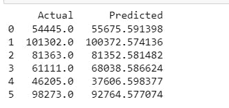
df_preds = pd.DataFrame({'Actual': y_test.squeeze(), 'Predicted': y_pred.squeeze()})
print(df_preds)
All of the anticipated values for the input values in the X test are now contained in the y pred variable. By putting the anticipated and actual output values for X test side by side in a dataframe structure, we can now compare them.

Evaluating the Model
from sklearn.metrics import mean_absolute_error, mean_squared_error
import numpy as np
mae = mean_absolute_error(y_test, y_pred)
mse = mean_squared_error(y_test, y_pred)
rmse = np.sqrt(mse)
print(f'Mean absolute error: {mae:.2f}')
print(f'Mean squared error: {mse:.2f}')
print(f'Root mean squared error: {rmse:.2f}')
