Time Series Store-sales Data

Code: kaggle.com/code/uom190649f/time-series-data..

Introduction

In this blog, we are going to present a solution to predict grocery sales with machine learning. We will forecast store sales using time-series forecasting based on data from Corporación Favorita, a big Ecuadorian supermarket retailer. We'll specifically create a model that more reliably predicts unit sales for thousands of goods sold at various Favorita locations. The reason we are doing this is because more precise forecasting in grocery shopping is more possible. Otherwise, businesses can get drawbacks due to overstocking.

Solution

Data Analysis

First of all we should install necessary Python libraries and import out dataset to the notebook.

import numpy as np # linear algebra
import pandas as pd # data processing, CSV file I/O (e.g. pd.read_csv)

# Input data files are available in the read-only "../input/" directory
# For example, running this (by clicking run or pressing Shift+Enter) will list all files under the input directory

import os
for dirname, _, filenames in os.walk('/kaggle/input'):
    for filename in filenames:
        print(os.path.join(dirname, filename))

Decomposing a time series entails seeing it as a collection of level, trend, seasonality, and noise components. Decomposition is a useful abstract paradigm for thinking about time series in general, as well as for better comprehending challenges in time series analysis and forecasting. It offers a systematic way of approaching a time series forecasting challenge, both in terms of modeling complexity in general and especially in terms of how to effectively represent each of these components in a given model. The statsmodels library provides an implementation of the naive, or classical, decomposition method in a function called seasonal_decompose().

import plotly.express as px
import seaborn as sns
import matplotlib.pyplot as plt

sns.set(color_codes=True)        
plt.style.use("seaborn-whitegrid")

from statsmodels.tsa.seasonal import seasonal_decompose

To be able to plot our data we will need more libraries such as plotly, seaborn and matplotlib as well.

Now, we can display our data.

df_train = pd.read_csv('/kaggle/input/store-sales-time-series-forecasting/train.csv',parse_dates=['date'])
df_train.head()

df_test = pd.read_csv('/kaggle/input/store-sales-time-series-forecasting/test.csv',parse_dates=['date'])
df_test.head()

Let's see the shape of our data to have a better understanding. It is often useful to know what shape your data takes because it gives clues about its descriptive features.

df_sub.shape

Let's import all other datasets as well.

df_oil=pd.read_csv('/kaggle/input/store-sales-time-series-forecasting/oil.csv',parse_dates=['date'])
df_holi=pd.read_csv('/kaggle/input/store-sales-time-series-forecasting/holidays_events.csv',parse_dates=['date'])
df_stores=pd.read_csv('/kaggle/input/store-sales-time-series-forecasting/stores.csv')
df_trans=pd.read_csv('/kaggle/input/store-sales-time-series-forecasting/transactions.csv',parse_dates=['date'])

Let's display these datasets as well and check out their shapes.

df_oil.head()

df_holi.head()

df_stores.head()

df_train.shape,df_test.shape,df_sub.shape,df_oil.shape,df_holi.shape,df_stores.shape,df_trans.shape

We should define "start" and "end" dates from our "date" column.

# full calendar set 
# create calender set 
cal_start = '2013-01-01'
cal_end =  '2017-08-31'
calendar = pd.DataFrame(index = pd.date_range(cal_start,cal_end)).to_period('D')
calendar.head()

Train and Test datasets¶

Handling Missing Values

Missing data happens in practically all research, even in well-designed and controlled studies. Missing data can diminish a study's statistical power and provide skewed estimates, resulting in invalid conclusions.

df_train.head()

df_train.shape

df_train.isna().sum()

df_test.isna().sum()

We will display the unique values.

df_train.store_nbr.unique()

Let's check the correlation. Spearman rank correlation is a non-parametric test that is used to determine the degree of relationship between two variables.

df_train.corr('spearman').sales.loc['onpromotion']

It should be around 0.5 We will use the groupby function to organize massive quantities of data and then perform actions on these groups.

df_train_family_on_sales = df_train.groupby(["date", "family"]).sales.sum().reset_index()
df_train_family_on_sales

Let's see how columns look with datatypes now.

df_train.info()

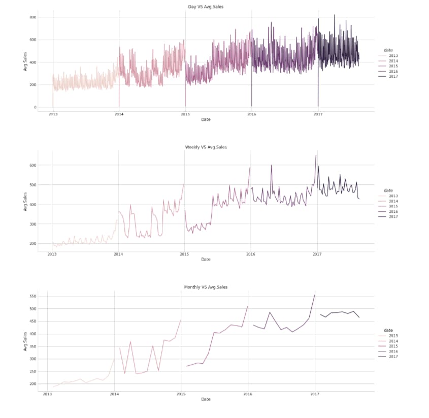
Average Sales on Date

We should see a concise summary of a DataFrame.

# df_eda.info()

df_eda = df_train.copy()
# df_eda.head()
df_eda=df_eda.set_index('date')

daily_sales=df_eda.resample('D').sales.mean().to_frame()  
weekly_sales=df_eda.resample('W').sales.mean().to_frame() 
monthly_sales=df_eda.resample('M').sales.mean().to_frame()  

df_sales=[daily_sales,weekly_sales,monthly_sales]
titles=['Day VS Avg.Sales','Weekly VS Avg.Sales','Monthly VS Avg.Sales']

for df,title in zip(df_sales,titles):

    sns.relplot(x=df.index,y=df.sales,kind='line',aspect=3,hue=df.index.year)
    plt.xlabel('Date')
    plt.ylabel('Avg.Sales')
    plt.title(title)

plt.show()

It should look like this:

Again, we should organize df_eda with groupby function.

temp=df_eda.groupby(df_eda.index.day_of_week)['sales'].mean().to_frame()
temp.head()

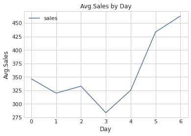
We should investigate how average sales change with the "day" label.

sns.lineplot(data=temp)
plt.xlabel('Day')
plt.ylabel('Avg.Sales')
plt.title('Avg.Sales by Day')
plt.show()

Sesonality trend analysis

avg_sales=df_eda.groupby('date').sales.mean()
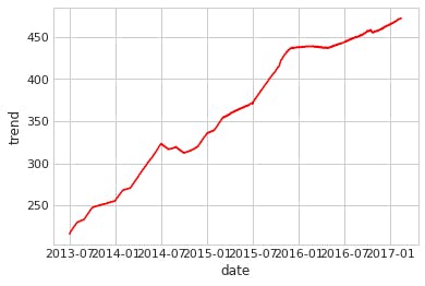
result = seasonal_decompose(avg_sales,model='additive',period=365)

Trend

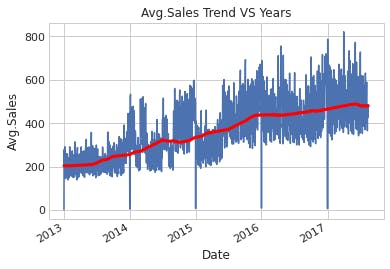
moving_avg=avg_sales.rolling(window=365,min_periods=183,center=True).mean()

ax=sns.lineplot(data=avg_sales)
ax=moving_avg.plot(color='red',linewidth=3)
plt.xlabel('Date')
plt.ylabel('Avg.Sales')
plt.title('Avg.Sales Trend VS Years')
plt.show()

So, there is a clear trend that we can observe.

sns.lineplot(data=result.trend,color='red')

Seasonal

sns.lineplot(data=result.seasonal)

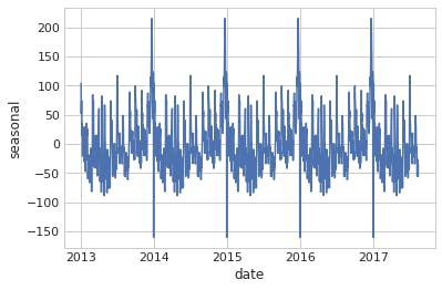
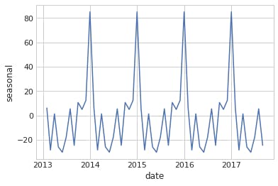
monthly_sales = seasonal_decompose(monthly_sales,model='addtive')
sns.lineplot(data=monthly_sales.seasonal)

result_weekly = seasonal_decompose(weekly_sales,model='addtive') sns.lineplot(data=result_weekly.seasonal)

![image.png](https://cdn.hashnode.com/res/hashnode/image/upload/v1667760422583/0YPIJUaEe.png align="left")

Oil dataset

It is time to investigate oil dataset.

df_oil.head()

df_oil.shape

We should deal with missing data in this dataset as well.

df_oil.isna().sum()

# sets the missing datas 
df_oil['date'] = pd.to_datetime(df_oil['date'])
df_oil = df_oil.set_index('date')['dcoilwtico'].resample('D').sum().reset_index()

We should observe a change in the shape here.

df_oil.shape

We will replace 0 with NaN

df_oil['dcoilwtico'] = np.where(df_oil['dcoilwtico']==0, np.nan, df_oil['dcoilwtico'])

df_oil.head()

Now, we should fill NaNs

# polynomial interpolation with order 2 
df_oil['dcoilwtico_intplo'] = df_oil.dcoilwtico.interpolate(method='polynomial',order=2)
df_oil.head()

df_oil.shape

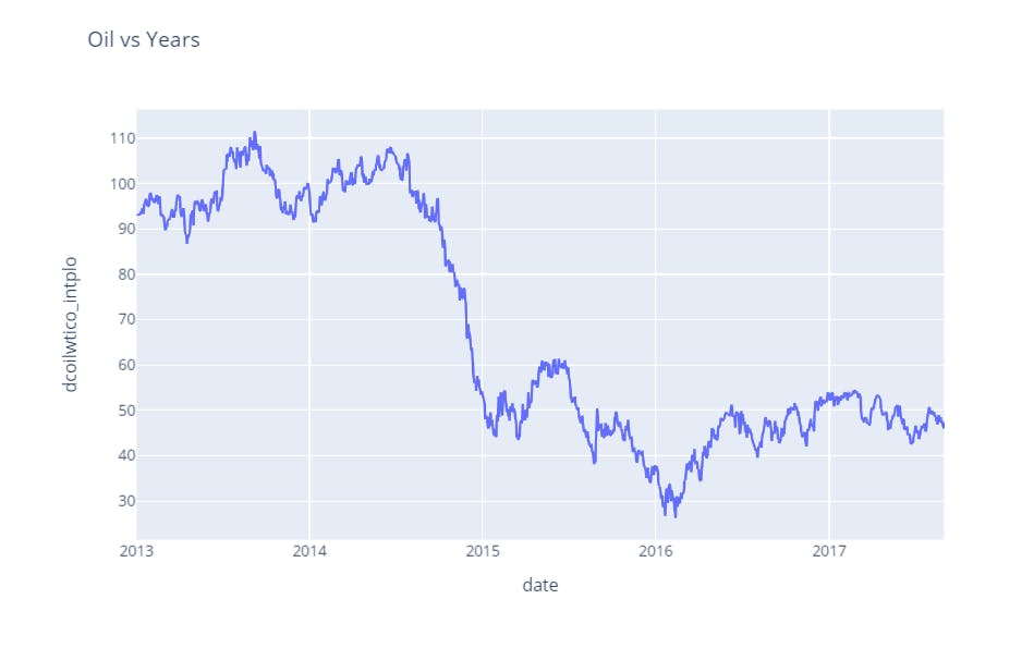
Let's plot our data.

px.line(df_oil, x='date',
        y='dcoilwtico_intplo',  title='Oil vs Years')

Sales on Oil

df_oil_2= df_oil.copy()
df_oil_2.set_index('date',inplace=True)
## merge oil dataset to eda dataset
df_eda_2 = df_eda.copy()
df_eda_2=pd.merge(left=df_eda_2,right=df_oil_2,left_index=True,right_index=True,how='left')
## Grouping by oil_price and date
avg_sales = df_eda_2.groupby(['date','dcoilwtico'])['sales'].mean().reset_index() 
# get the correlation value
np.round(avg_sales[['sales','dcoilwtico']].corr().iloc[0,1],4)

Let's display our data.

df_eda_2

Modelling

df_train_2 = df_train.copy()
df_train_2['date'] = df_train_2.date.dt.to_period('D')
df_train_2 = df_train_2.set_index(['date', 'store_nbr', 'family']).sort_index()
# df_train.head()
df_train_2_set_1 = df_train_2.copy()

train_start_date = '2017-04-30' 
train_end_date = '2017-08-15'

y = df_train_2_set_1.unstack(['store_nbr', 'family']).loc[train_start_date:train_end_date]
y.head()

We should import DeterministicProcess and CalendarFourier

from statsmodels.tsa.deterministic import DeterministicProcess, CalendarFourier
fourier = CalendarFourier(freq = 'W', order = 3)
dp = DeterministicProcess(index = y.index,
                          order = 1,
                          seasonal = True,
                          constant = False,
                          additional_terms = [fourier],
                          drop = True)
x = dp.in_sample()
x = x.join(calendar_2)
x.head()

Predicting for the next 16 days

x_test = dp.out_of_sample(steps = 16)
x_test = x_test.join(calendar_2)
x_test.head()

Training

from sklearn.metrics import mean_squared_log_error as msle
from sklearn.model_selection import TimeSeriesSplit
from sklearn.svm import SVR

from sklearn.ensemble import RandomForestRegressor

from sklearn.linear_model import LinearRegression
from sklearn.multioutput import MultiOutputRegressor

from sklearn.metrics import mean_absolute_error

Linear Model

lnr = LinearRegression(fit_intercept = True, n_jobs = -1, normalize = True)
lnr.fit(x, y)

yfit_lnr = pd.DataFrame(lnr.predict(x), index = x.index, columns = y.columns).clip(0.)
ypred_lnr = pd.DataFrame(lnr.predict(x_test), index = x_test.index, columns = y.columns).clip(0.)
y_ = y.stack(['store_nbr', 'family'])
y_['lnr'] = yfit_lnr.stack(['store_nbr', 'family'])['sales']
print('LNR MAE :', mean_absolute_error(y, yfit_lnr))

print('LNR RMSLE :', np.sqrt(msle(y, yfit_lnr)))

y_sub_lnr = pd.DataFrame(lnr.predict(x_test), index = x_test.index, columns = y.columns).clip(0.)
y_sub_lnr.head()

y_sub_lnr = y_sub_lnr.stack(['store_nbr', 'family'])
y_sub_lnr.head()

y_sub_lnr.shape

df_sub.shape

df_sub['sales'] = y_sub_lnr.values[:,2]
df_sub.head()

df_sub.to_csv('submission.csv', index = False)

SVR model

svr = MultiOutputRegressor(SVR(C = 0.2, kernel = 'rbf'), n_jobs = -1)
svr.fit(x, y)

yfit_svr = pd.DataFrame(svr.predict(x), index = x.index, columns = y.columns).clip(0.)
ypred_svr = pd.DataFrame(svr.predict(x_test), index = x_test.index, columns = y.columns).clip(0.)
print('SVR MAE :', mean_absolute_error(y, yfit_svr))

print('SVR RMSLE :', np.sqrt(msle(y, yfit_svr)))

y_sub_svr = pd.DataFrame(svr.predict(x_test), index = x_test.index, columns = y.columns).clip(0.)
y_sub_svr.head()

y_sub_svr = y_sub_svr.stack(['store_nbr', 'family'])
y_sub_svr.head()

df_sub['sales'] = y_sub_svr.values[:,2]
df_sub.head()

df_sub.to_csv('submission_2.csv', index = False)

Random Forest

rfr = RandomForestRegressor(n_estimators = 225, n_jobs=-1)
rfr.fit(x,y)

yfit_rfr = pd.DataFrame(rfr.predict(x), index = x.index, columns = y.columns).clip(0.)
ypred_rfr = pd.DataFrame(rfr.predict(x_test), index = x_test.index, columns = y.columns).clip(0.)
print('RFR MAE :', mean_absolute_error(y, yfit_rfr))

print('RFR RMSLE :', np.sqrt(msle(y, yfit_rfr)))

y_sub_rfr = pd.DataFrame(rfr.predict(x_test), index = x_test.index, columns = y.columns).clip(0.)
y_sub_rfr.head()

y_sub_rfr = y_sub_rfr.stack(['store_nbr', 'family'])
y_sub_rfr.head()

Combine

df_sub['sales'] = np.mean([y_sub_svr.values[:,2], y_sub_lnr.values[:,2],y_sub_rfr.values[:,2]],axis = 0)
df_sub.head()

df_sub.to_csv('submission_4.csv', index = False)